Lately, machine learning has become the buzzword in business community and rightly so due to the immense opportunities it offers. But one hurdle absolute beginners face is learning a new language like R or Python. Yes! they are absolutely necessary if you want to control and tune every single aspect of your workflow, But for beginners, quickly getting to something tangible is more important to keep up the enthusiasm of learning. Today I will go through one such tool- Orange - which is perfect for teaching machine learning to beginners without getting into nitty-gritty of programming.
What is Orange
Orange is a data visualization, machine learning and data mining toolkit with a visual programming front-end. It is open source and has been around since 1996. The analysis is done through connecting widgets which performs different functions like reading files, showing feature statistics, building models, evaluating etc. Moreover, it is available as a Python library if you intend to delve deeper into finer tuning.
Where do I get it
You can follow the installation instruction from the official website. It is also available with standard Conda distribution . Orange version 3.20.1 was used for this tutorial.
Our objective today
We are going to build a simple workflow to predict house prices based on a given dataset with a random forest model. We will be using the Kaggle House Prices dataset. As this is a beginner friendly tutorial, the objective is to demonstrate the workflow in Orange3 and churning out a model fast is first priority. Hence, we will not delve into the abyss of granular imputation (will use barebones imputation) ,feature engineering and hyperparameter tuning.
How it works
After launching Orange, you will be welcomed by the following screen. In the left are slew of widgets neatly organized in categories based on their purposes. The big white space is your playground where you drag and drop the widgets, connect and configure them to create your own workflow. Double-clicking on any widget will bring up its corresponding properties where you can tweak different parameters.

Loading data
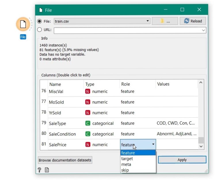
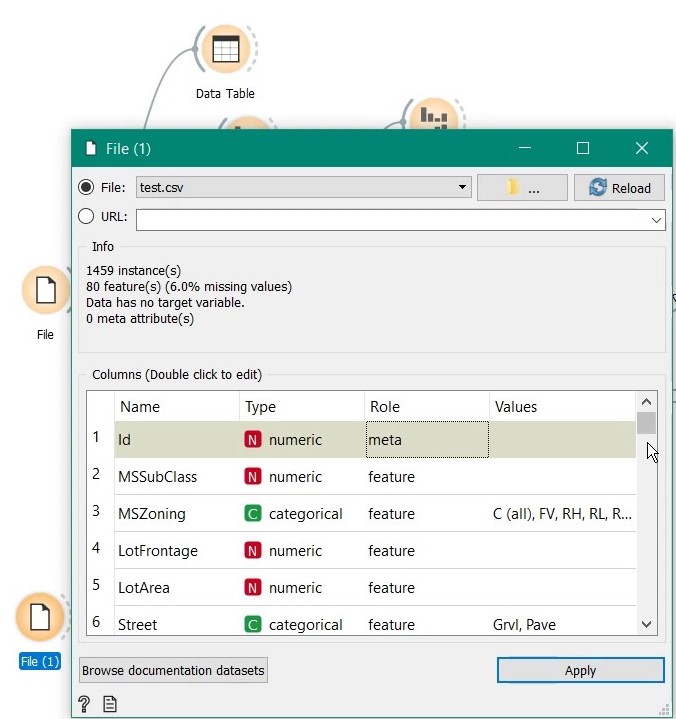
Just drag the File widget into workspace, double click to open the properties and select the training dataset. That’s it, data is loaded and you can see the features at the bottom. The variable which we want to predict is SalePrice. Scroll down and select its role as target.
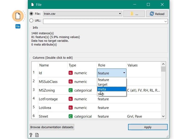
Then change the role of id variable to meta as it just not a predictor, just tag for identification.
Exploring the data
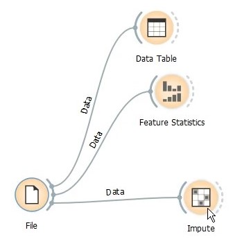
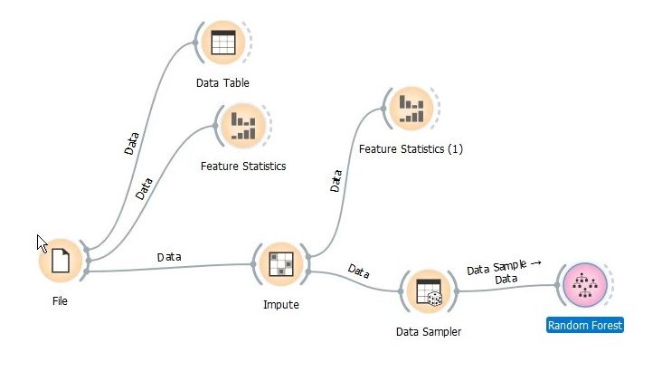
We drag to more widgets - Data Table and Feature Statistics and connect with our loaded data. Data Table shows the data you loaded.
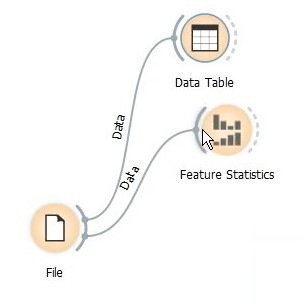
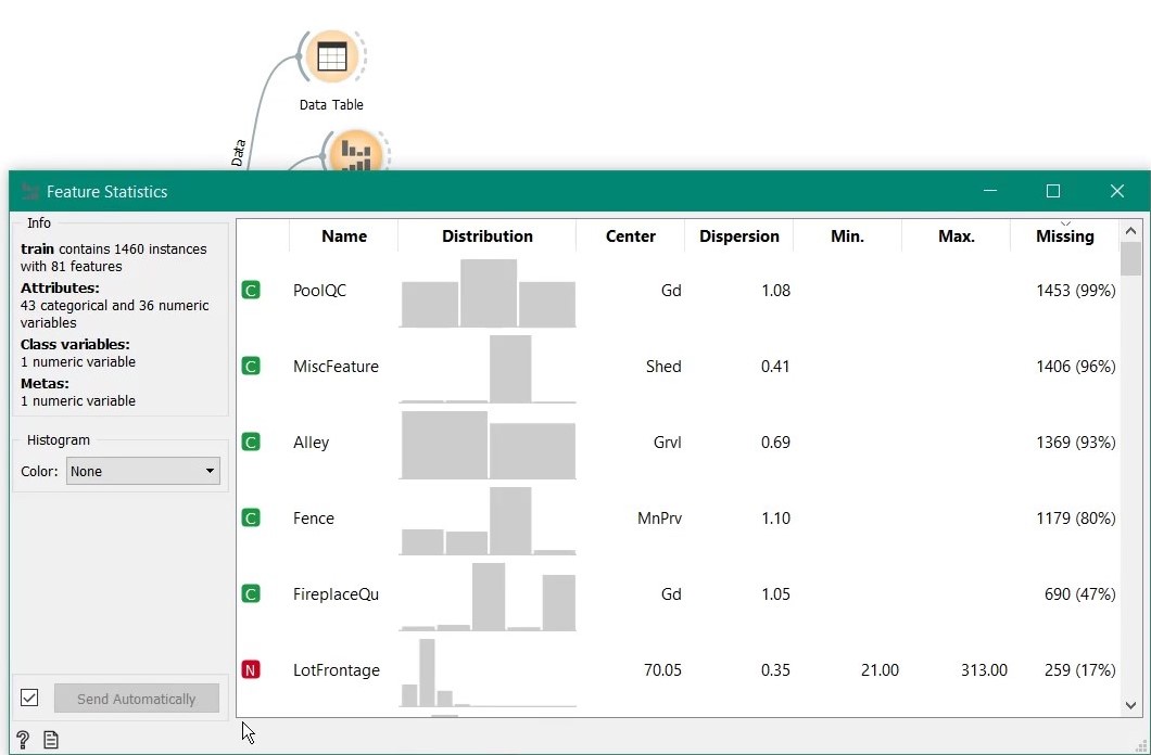
Feature statistics widget shows handy details on each column. We observe that lots of data are missing.
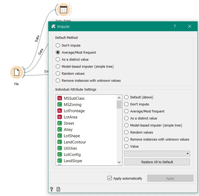
Let’s do some imputation. Drag the Impute widget and connect it with the data.
As said earlier, we will do barebones (aka the easy way out) imputation by taking average values if missing value is numeric and most frequent value if it is categorical. Of course, orange is capable of handling each feature individually and different imputation techniques are essential for a better model. But for this tutorial, we will stick to simple.
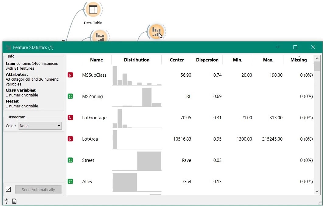
After imputation, again we drag another Feature Statistics widgets and connect it to the output of Impute widget. As we can see, no more missing values.
Building the model
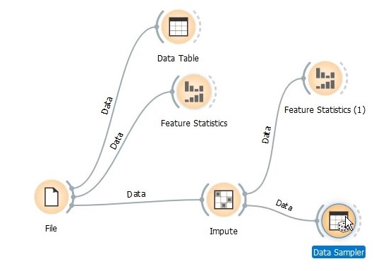
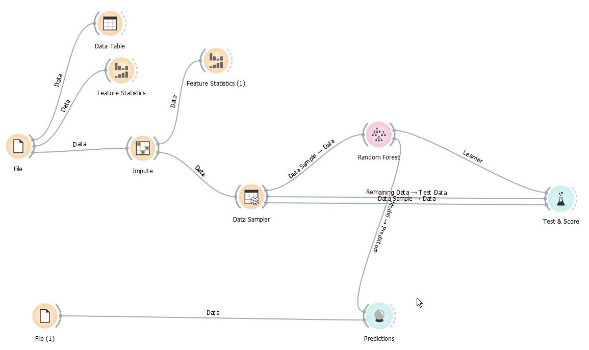
Before going for predictions with the test set, we are going to divide the training data for validation. For this we add a new widget Data Sampler.
In the Data Sampler properties, you can specify different sampling type. For simplicity of understanding, I have gone for fixed partitioning but k-fold cross validation is more robust and likely to yield better results.
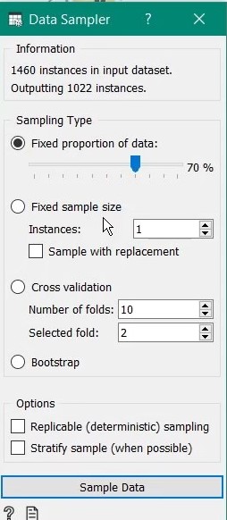
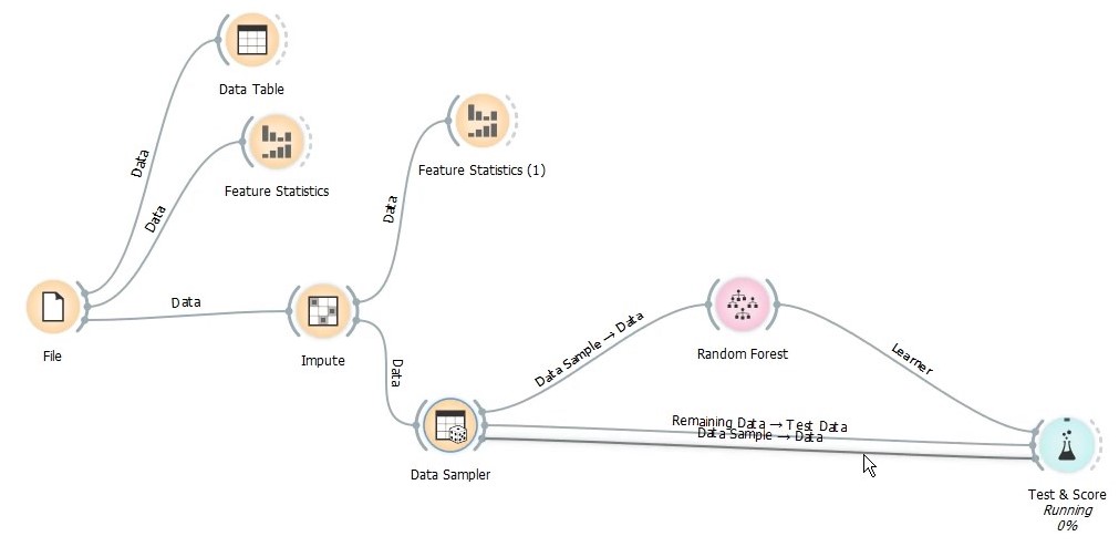
Data sampler outputs two separate datasets - data sample which will be used to train a model/learner and remaining data will be used as validation set. Next, we drag the Random Forest learner and connect data sample to it. The random forest learner contains several parameters to tune like number of trees, tree depth, minimum child tree size etc. I have set the maximum number of trees to 200 and minimum child tree size to 10 for this exercise.
After that, we add Test & Score widget which is used to evaluate our learner’s performance against the validation dataset we created from by Data Sample. In the widget, learner goes as model input, data sample as train data and remaining data as test data/validation set.
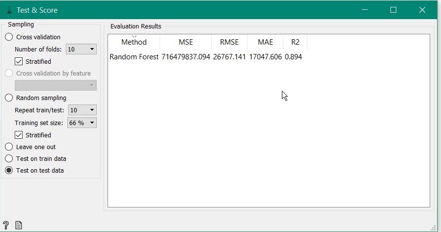
Double clicking the Test & Score reveals the model evaluation metrics like RMSE, R-squared etc. Judging by the results, it seems a decent enough model considering little to no imputation and feature engineering done.
Predicting the unknown
Now that our model is done, let’s predict based on test data. Again, we load train data through File widget and change id to meta.
Next, we directly connect the test data to a new widget called Predictions which does the magic of predicting. We also connect our Random Forest learner output as the model to use for predictions.
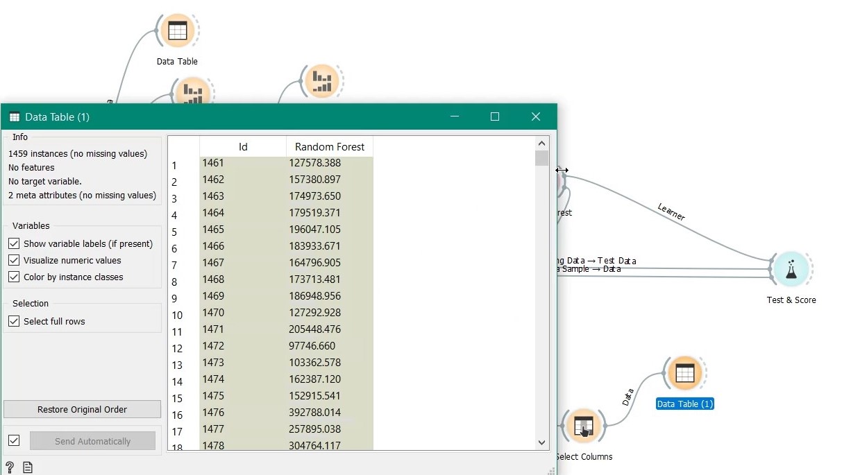
That’s it our prediction is done. We add another widget Select Columns to get only the predictions against id and use Data Table to view the results as below.
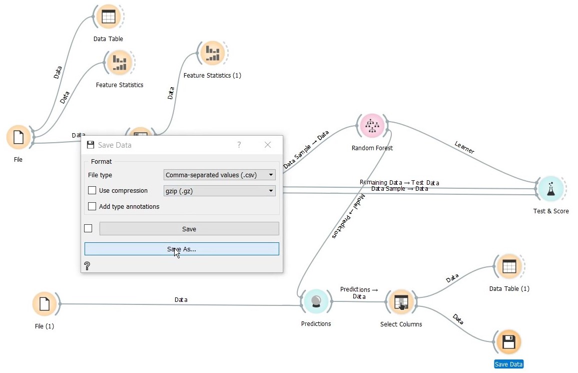
By adding the Save Data widget we can save the data in different formats.
Results
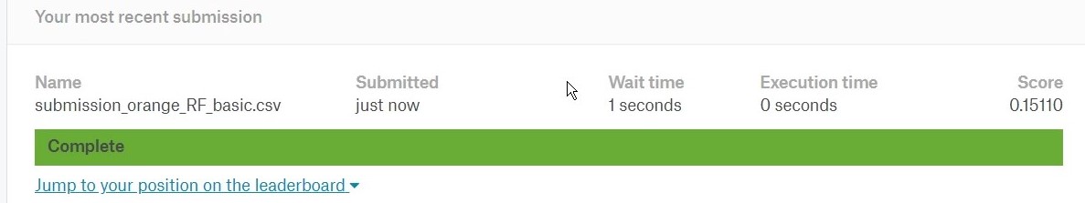
Although it was a pretty weak model building where we skipped many major steps, our model did decent in the Kaggle leaderboard with a score of 0.15110 which places it at around 3000th among 4700 submissions at the time of writing.
Final thoughts
As we have seen in this tutorial, it does not take whole lot of programming prowess to churn out a machine learning model but if you want to improve the model further it requires granular control on every component and there comes the programming chops and statistical know-how. For the keen explorers who wants to delve deeper to further improve the model, looking at the following will return great dividends-
- Imputation - Consider interaction between different variables
- Feature elimination- Lots of features in the data show multi-collinearity. Keeping the relevant ones will do wonders.
- Hyperparameter tuning - Although Orange is limited in this regard, further examination likely to yield better outcomes
Sharing is caring. Share this story in...
Share: Twitter Facebook LinkedIn Pocket Flipboard